Rotary Position Embeddings (RoPE)

Attention by itself has no idea of order: shuffle the tokens and every attention score stays the same. The model has to be told where each token is.

The classic way: a learned table

The classic model keeps a table with one learned vector per position and adds it to the token embedding:

x = self.token_embed(idx) + self.position_embed(self.pos_idxs[:T])

This works, with three weaknesses:

1. Positions the model never trained on have random vectors. The legacy config trains on 16-token windows with a 512-position table, so positions 16 to 511 stay untrained, and generating past 16 tokens feeds the model noise. (generate_text.py now stays inside the trained window for exactly this reason.)
2. The model must learn from data that position 7 next to position 8 means the same as 107 next to 108. Absolute positions make relative order a learned fact.
3. The table costs context_length x n_embed parameters.

The rotary way

RoPE does not touch the embeddings. Inside attention, it rotates each query and key vector by an angle proportional to its position. Split a head vector of size d into d/2 pairs. Pair i of a token at position m is rotated by the angle m * theta_i, with

\[ \theta_i = \text{rope\_theta}^{-2i/d}, \qquad i = 0, 1, \ldots, d/2 - 1 \]

\[ \begin{pmatrix} x'_{i} \\ x'_{i + d/2} \end{pmatrix} = \begin{pmatrix} \cos m\theta_i & -\sin m\theta_i \\ \sin m\theta_i & \cos m\theta_i \end{pmatrix} \begin{pmatrix} x_{i} \\ x_{i + d/2} \end{pmatrix} \]

The key property: a rotation by angle a followed by the dot product with something rotated by angle b only depends on a - b. So the attention score between a query at position m and a key at position n depends only on the distance m - n:

\[ \langle R_m q,\; R_n k \rangle = \langle q,\; R_{n-m}\, k \rangle \]

Attention now sees relative positions directly and there are no position parameters to train. It does not make long contexts free, though: a model trained on 512-token windows has never seen two tokens 2,000 positions apart, and the section on rope_theta below is about exactly that.

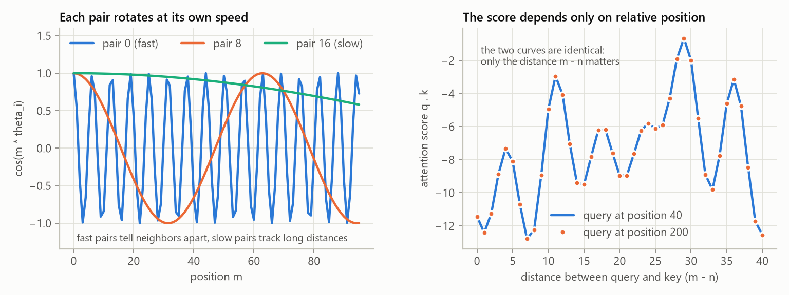
The left plot shows why the frequencies are spread out. Early pairs spin fast (they tell neighbors apart), late pairs spin slowly (they still distinguish tokens thousands of positions apart). The right plot is the property above, measured: the score between a fixed query and key only depends on how far apart they are, wherever the pair sits.

The code

def rope_cache(dim, max_len, theta=10_000.0):
    positions = torch.arange(max_len, dtype=torch.float32)
    angles = torch.outer(positions, rope_frequencies(dim, theta))    # (max_len, dim/2)
    return angles.cos(), angles.sin()

def apply_rope(x, cos, sin):                                         # x: (..., seq, dim)
    half = x.shape[-1] // 2
    x1, x2 = x[..., :half], x[..., half:]
    return torch.cat([x1 * cos - x2 * sin, x1 * sin + x2 * cos], dim=-1)

The tables are computed once and stored as non-persistent buffers, so they are not saved in checkpoints. With a KV cache, the new token at position p uses row p of the tables, which is why forward_hidden slices rope_cos[start : start + T].

The pairs here are (x[i], x[i + d/2]) (the "rotate half" layout used by most open code). Meta's original Llama code pairs neighbors (x[2i], x[2i+1]) instead. The two are the same up to a fixed permutation of the dimensions, which the projection weights absorb.

Two tests pin the math: test_rope_is_a_rotation_of_each_pair compares every pair with an explicit 2x2 rotation matrix, and test_rope_scores_depend_only_on_relative_position checks the property above.

Longer contexts and rope_theta

rope_theta sets the slowest frequency. The default 10,000 comes from the original paper. Models with long contexts raise it (Llama 3 uses 500,000), which slows every pair down. With 64 pairs per head and a 128K-token context, no pair turns less than once across the whole context at 10,000, while 15 of them do at 500,000, and those slow pairs are what can tell far-apart positions apart. Methods that stretch a trained model to longer contexts (position interpolation, NTK scaling, YaRN) all work by rescaling these frequencies, which is easy precisely because positions live in one small function.

DeepSeek's multi-head latent attention uses RoPE on only a small part of each head (the "decoupled" key); see attention for why.